Johns Hopkins Turbulence Databases

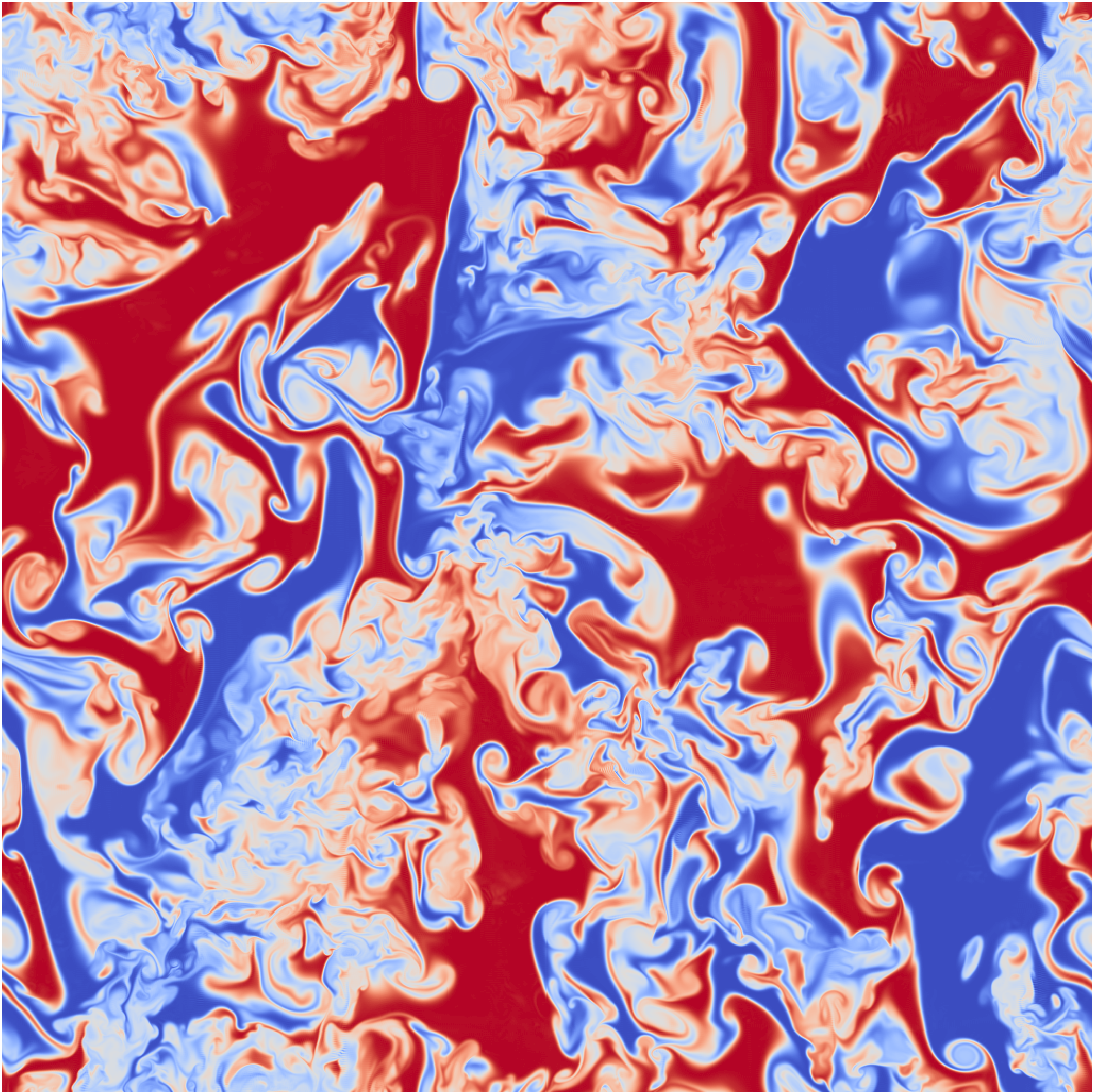
Dataset description

Homogeneous buoyancy driven turbulence:

Simulation data provenance: Los Alamos National Laboratory using the LANL DNS code (see README-HBDT for more details).

• Direct Numerical Simulation (DNS) of homogeneous buoyancy driven turbulence in a domain size 2π × 2π × 2π, using 1,024³ nodes.
• The incompressible two-fluid Navier-Stokes equations are solved using a pseudo-spectral method. These equations represent the large speed of sound limit for the fully compressible Navier-Stokes equations with two fluids having different molar masses and obeying the ideal-gas equation of state.
• The domain is triply periodic and the homogeneity of the fluctuating quantities is ensured by imposing mean zero velocity and constant mean pressure gradient. These conditions are similar to those encountered in the interior of the Rayleigh-Taylor mixing layer.
• The two fluids are initialized as random blobs, with a characteristic size of about 1/5 of the domain. The flow starts from rest, in the presence of a constant gravitational acceleration, and the fluids start moving in opposite direction due to differential buoyancy forces. Turbulence fluctuations are generated and the turbulent kinetic energy increases; however, as the fluids become molecularly mixed, the buoyancy forces decrease and at some point the turbulence starts decaying.
• Due to the change in specific volume during mixing, the divergence of velocity is not zero, but related to the density field. This leads to a variable coefficient Poisson equation for pressure, which is decomposed in two parts, for the gradient and curl components of ∇p/ρ. These are solved using direct solvers to ensure mass conservation and baroclinic generation of vorticity to machine precision.
• The 1015 time frames stored in the database cover both the buoyancy driven increase inturbulence intensity as well as the buoyancy mediated turbulence decay. Each time frame contains the density, 3 velocity components, and pressure at the grid points. The frames are stored at a constant time interval of 0.04, which represents between 20 to 50 DNS time steps.
• Schmidt number: 1.0
• Froude number: 1.0
• Atwood number: 0.05
• Maximum turbulent Reynolds number: Re_τ ~ 17,765.
• Minimum turbulent Reynolds number during decay phase: Re_τ ~ 1,595.
• A file with the time history of the Favre turbulent kinetic energy, k^˜ = <ρu_i^''u_i^''> ⁄ 2<ρ>, Reynolds stresses, R_ii = <ρu_i^''u_i^''> (no summation over i), vertical mass flux, a_v = <ρ u₁^'> ⁄ <ρ>, turbulent Reynolds number, Re_t = k^˜2 ⁄ νε, eddy turnover time, τ = k^˜ ⁄ ε, kinetic energy dissipation, ε, density variance and density-specific volume correlation can be found here. (Note: Until July 22, 2015, the time-history file that was posted on this site included the total kinetic energy instead of the Favre turbulent kinetic energy. The file posted since July 22, 2015 lists the Favre turbulent kinetic energy)
• Files with tables of the power spectra of density, 3 velocity components, and mass flux can be downloaded at the following times: 6.56, 11.4, 15.0, 20.0, 30.0, and 40.0.
• Files with tables of the density PDF can be downloaded for the following times: 0.0, 6.56, 11.4, 15.0, 20.0, 30.0, and 40.0.